Is Tensor Flow Easy to Learn if You Never Coded Before

Getting started with Tensorflow

Learn the basics through examples

Photo by Marten Newhall from Unsplash.

Introduction

Ok, let's discuss the elephant in the room. Should you learn Tensorflow or PyTorch?

Honestly, there is no right answer. Both platforms have a large open source community behind them, are easy to use, and capable of building complex deep learning solutions. If you really want to shine as a deep learning researcher you will have to know both.

Let's now discuss how Tensorflow came about and how to use it for deep learning.

When was Tensorflow developed ?

Artificial Neural Networks (ANN) research has been around for a long time. One of its earlier works was published by Waren McCulloch and Walter Pitts in 1943 where the authors developed one of the first computational models for ANNs¹.

Prior to the early 2000s only rough frameworks were available and experienced ML practitioners were required to build simple / moderate ANN approaches².

With the surge interest in ANNs in 2012³ the landscape in Deep Learning (DL) frameworks started to change. Caffe, Chainer and Theano were arguably the top contenders in the early days and made the use of DL easier for the average Data Scientist.

Google searches for the top low/high level deep learning frameworks between January 2012 and July 2021 under the 'Machine Learning & Artificial Intelligence' category. Image from the author.

In February 2015, Google open sourced Tensorflow 1.0 and this framework quickly gained traction. Tensorflow swift adoption can be linked to a few factors such as a strong household name, fast and frequent updates, simple syntax and focus on availability and scalability (e.g. mobile and embedded devices)⁴⁵.

With the increased popularity of PyTorch and reduced market share of Tensorflow⁶, the Google team released in 2019 a major update to the library "Tensorflow 2.0"⁷. This update introduced eager execution (one of the key selling points of PyTorch), as well as natively supporting Keras (greatly simplifying development through static computational graphs).

By June 2021, more than 99% of the Google searches for major deep learning frameworks contained either Tensorflow, Keras or PyTorch.

Learning through examples

The simplest way to learn (at least for me) is through examples. This approach allows you to test a working process, modify it, or take components which are useful for your project.

In this blog, I'll be guiding you through two ML examples, illustrating the key components needed to build simple Tensorflow models.

To facilitate replicability I suggest using Google Colab for the examples described here. To do so, simply open this link and follow the steps to create a new python 3 notebook.

Linear regression

In this example, we will build a simple 1 layer Neural Network to solve a linear regression problem. This example will explain how to initialise your weights (aka the regression coefficients), and how to update them through backpropagation.

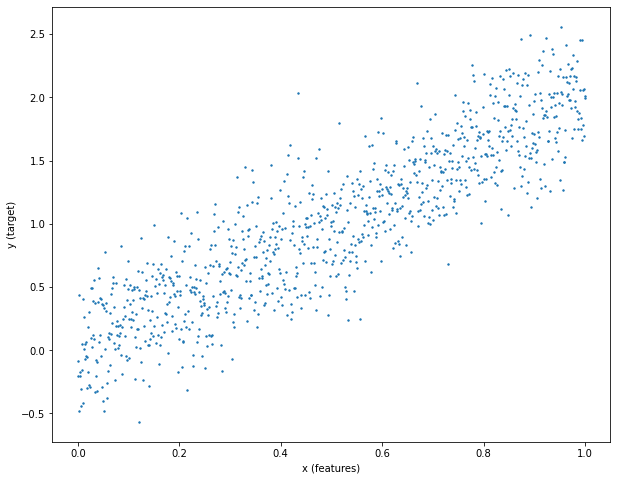
The first thing we need is a dataset. Let's simulate a noisy linear model as

where Y is our target, X is our input, w is the coefficient we want to determine, and N is a Gaussian distributed noise variable. To do so, in the first cell of your notebook paste and run the following snippet.

This will display a scatter plot of the relation between X and Y, clearly indicating a linear correlation under some Gaussian noise. Here, we would expect a reasonable model to estimate 2 as the ideal regression coefficient.

Simulated data representing a linear correlation between X and Y under Gaussian noise.

Let's now initiate our regression coefficient (here on called weight) with a constant number (0.1). To do this we first need to import the Tensorflow library, then initialise the weight as a Tensorflow variable.

For the purpose of this example, assume a Variable to have similar properties to a Tensor. A tensor is a multidimensional array of elements represented by a tf.Tensor object. A tensor has a single data type (in the following example 'float32') and a shape. This object allows other Tensorflow functions to perform certain operations such as calculating the gradient associated to this variable and updating its value accordingly. Copy the following snippet to initialise our weight variable.

Running this snippet will output the variable name, shape, type and value. Note that this variable has a '()' shape indicating that its a 0 dimensional vector.

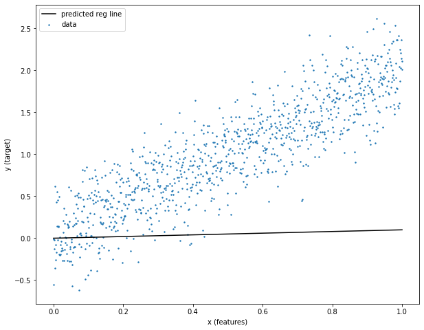
          <tf.Variable 'Variable:0' shape=() dtype=float32, numpy=0.1>        

To obtain the predicted Y (Yhat) given the initialised weight tensor and the input X we can simply call `Yhat = x * w_tensor.numpy()`. The '.numpy()' is used to convert the weight vector to a numpy array. Copy and run the following snippet to see how the initialised weight fits the data.

As you can observe the current value of 'w_tensor' is far from ideal. The regression line does fit the data at all.

Representation of the model fit prior to training.

To find the optimal value for 'w_tensor' we need to define a loss metric and an optimiser. Here, we will use the Mean Squared Error (MSE) as our loss metric, and the Stochastic Gradient Descent (SGD) as our optimiser.

We now have all the pieces in place to optimise our 'w_tensor'. The optimisation loop simply requires the definition of the 'forward step' and a call to the minimize function from our optimiser.

The 'forward step' tells the model how to combine the input with the weight tensor and how to calculate the error between our target and the predicted target (line 5 in the snippet below). In a more complex example, this would be a set of instructions that define the computational graph from the input X to the target Y.

To minimise the defined loss we simply need to tell our optimiser to minimise the 'loss' in respect to our 'w_tensor' (line 17 in the snippet below).

Add the following snippet to your example to train the model for 100 iterations. This will dynamically plot the new weight value and the current fit.

By the end of the train loop your weight should be reasonably close to 2 (ideal value). To use this model for inference (i.e. to predict the Y variable given an X value) you can simply do `Yhat = x * w_tensor.numpy()`

Representation of the model fit after training.

Classification problem

In this example, we will introduce the Keras Sequential model definition to create a more complex Neural Network. We will apply this model to a linearly separable classification problem.

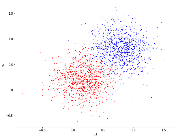
As before, let's start by building our dataset. In the snippet below, we create two clusters of points centered at (0.2, 0.2) for the first cluster, and (0.8, 0.8) for the second cluster.

We can quickly observe that a model that linearly separates the two datasets by a line at equal distance to both clusters would be ideal.

Simulated data representing two clusters of data, with the first cluster centered at (0.2, 0.2) and the second cluster centered at (0.8, 0.8).

As before, let's define our loss metric and optimizer. In this example we should use a classification loss metric such as the Cross Entropy. Since our target is encoded as an integer we must use the 'SparseCategoricalCrossEntropy' method.

For the optimizer we could use the SGD as before. However, the vanilla SGD is incredibly slow to converge. Instead, we will use a more recent adaptive gradient descent approach (RMSProp).

The next step is to define the custom NN model. Let's create a 5 layer neural network as follows:

1. Linear layer with 10 nodes. This will have a shape of 2 x 10 (input_shape x layer_size).
2. Batch Normalisation layer. This layer will normalise the output of the first layer for each batch, avoiding exploding / vanishing gradients.
3. Relu activation layer. This layer will provide a non-linear capability to our network. Note that we only use this as an example. A relu layer is unnecessary for this problem as it is linearly separable.
4. Linear layer with 2 nodes. This will have a shape of 10 x 2 (layer_size x output_shape).
5. Softmax layer. This layer will convert the output from layer 4 into a softmax.

Before the network can be used for training we need to call the 'compile' method. This will allow Tensorflow to link the model to the optimizer and the loss metric defined above.

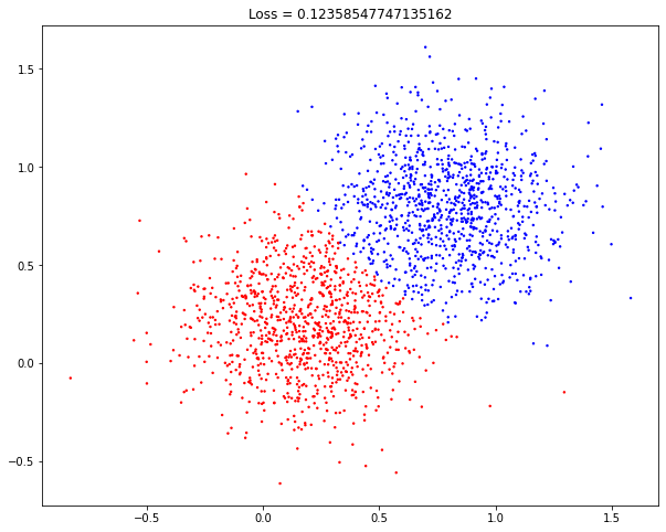
As before, let's first check how our network performs before training. To use the model for inference we can simply type 'yhat = model.predict(x)'. Now, copy the snippet below to visualise the network output.

As you can confirm the network is not good at all. It clearly needs some training to properly separate the two classes.

Representation of the model fit prior to training.

To train a Keras model we can simply type 'model.fit(x, y, epochs=50)'. Add the snippet below to your notebook to train the model.

By the end of the train loop your network should be reasonably good at separating both classes. To use this model for inference (i.e. to predict the Y variable given an X value) you can simply do `yhat = model.predict(x)`.

Representation of the model fit after training.

Complete script

For the full script go to my Github page by following this link:

Or go directly to the Google Colab notebook by following this link:

Conclusion

Tensorflow is one of the best deep learning frameworks right now to develop custom deep learning solutions. In this blog, I introduced the key concepts to build two simple NN models.

Warning!!! Your learning just started. To get better you will need to practice. The official Tensorflow website provides a good source of examples from beginner to expert level, as well as the official documentation to the Tensorflow package. Good Luck!

bastienhavine.blogspot.com

Source: https://towardsdatascience.com/getting-started-with-tensorflow-e33999defdbf

Share this post